Authored by Tony Feng
Created on Feb 10nd, 2022
Last Modified on Feb 10nd, 2022
Intro
This sereis of posts contains a summary of materials and readings from the course CSCI 1430 Computer Vision that I’ve taken @ Brown University. This course covers the topics of fundamentals of image formation, camera imaging geometry, feature detection and matching, stereo, motion estimation and tracking, image classification, scene understanding, and deep learning with neural networks. I posted these “Notes” (what I’ve learnt) for study and review only.
Definition
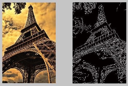
The process of identifying parts of a digital image with sharp changes (discontinuities) in image intensity.
It is helpful to:
- Recognize objects
- Reconstruct scenes
- Edit images (artistically)
- Recover geometry and viewpoint
Causes of Edges
- Surface orientation discontinuity
- Physical edges in the 3D object
- Depth discontinuity
- Viewing objects from a certain perspective
- Surface color discontinuity
- Differences in colors between
- Illumination discontinuity
- Lighting and shadows
Characterizing Edges
Gradient
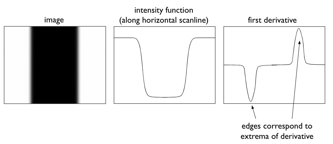
Simple algorithm for edge detection is to find gradient. The first derivative is strongest (i.e. has the highest magnitude) where the intensity changes most rapidly. The sign of the derivative depends on whether the intensity falls from high to low or rises from low to high.


Effects of Noise
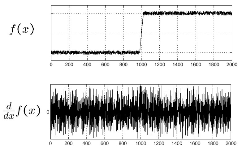
Real images are noisy, which results in lots of noise in the first derivative and starts to overwhelm the peaks. It would be almost impossible to detect where the edge occurred by inspecting the derivative graph with all that noise.

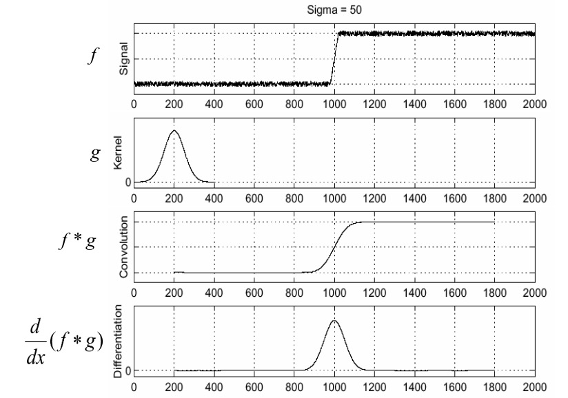

We can fix this by filtering the signal (image) first to smooth out the noise before computing the derivative. Here, a gaussian filter is common. To find edges, look for peaks in $\frac{\mathrm{d}}{\mathrm{d} x}(f*g)$
Derivative Theorem
$$\frac{d}{d x}(f * g)=f * \frac{d}{d x} g$$
This means that we can compute the derivative just on the filter $g$ and convolve the image by the differentiated filter to get the same result. Instead of convolving the image twice (once to denoise and once to compute the derivative), we only need to convolve once.
Tradeoff
Smoothed derivative removes noise, but blurs edge, also finds edges at different frequencies. The bigger the kernel, the more smoothed out the edges of the image are since we start removing lower frequencies.

Designing an Edge Detector
Criteria
- Good detection
- Finding all real edges
- Ignoring noise or other artifacts
- Good localization
- The edges detected must be as close as possible to the true edges
- Returning one point only for each true edge point
Cues of Edge Detection
- Differences in color, intensity, or texture across the boundary
- Continuity and closure
- High-level knowledge
Canny Edge Detector
- Filter image with $x$, $y$ derivatives of Gaussian
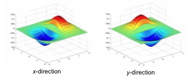
- Find magnitude and orientation of gradient
$$ |G| =\sqrt{G_{x}^{2}+G_{y}^{2}} $$ $$\theta(x, y) =\arctan \left(\frac{G_{y}}{G_{x}}\right)$$
- Non-maximum Suppression e.g. Bilinear Interpolation
- ‘Hysteresis’ Thresholding
- Define two thresholds: low and high
- Grad. mag. > high threshold = strong edge
- Grad. mag. < low threshold = noise
- In between = weak edge
- Use the high threshold to start edge curves
- Use the low threshold to continue them into weak edges
- ‘Follow’ edges starting from strong edge pixels
- Define two thresholds: low and high

