Authored by Tony Feng

Created on Feb 10nd, 2022

Last Modified on Feb 14nd, 2022

Intro

This sereis of posts contains a summary of materials and readings from the course CSCI 1430 Computer Vision that I’ve taken @ Brown University. This course covers the topics of fundamentals of image formation, camera imaging geometry, feature detection and matching, stereo, motion estimation and tracking, image classification, scene understanding, and deep learning with neural networks. I posted these “Notes” (what I’ve learnt) for study and review only.

Overview

Edges and corners are typically called features that are unique to some part of the image. Local features describe one component of the image, not the entirely image.

Corners are also called interest points or key points.

Corners are important, because we can get spare correspondences, which allows for fast matching between images.

Finding distinctive and repeatable feature points can be difficult when we want our features to be invariant to large transformations:

• geometric variation (translation, rotation, scale, perspective)
• appearance variation (reflectance, illumination)

Example: Panorama Stitching

Using panorama requires correspondences. We have two images of a scene, and we can see that there is some overlay, but the images are not quite the same.

We need our features/corners to have some sort of properties in this case: 1) distinctiveness, 2) repeatability, 3) compactness, 4) efficiency.

Local Feature Matching

• Detection
  • Find a set of distinctive features (e.g. key points, edges)
• Description:
  • Extract feature descriptor around each interest point as vector.
• Matching:
  • Compute distance between feature vectors to find correspondence.

Corner Detection

Basic idea

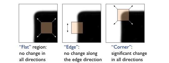
We do not know which other image locations the feature will end up being matched against. But we can compute how stable a location is in appearance with respect to small variations in its position. In other words, we can compare image patch against local neighbors.

We want a window shift in any direction to give a large change in intensity.

Auto-correlation

$$E(u, v)=\sum_{x, y} w(x, y)[I(x+u, y+v)-I(x, y)]^{2}$$

, where $w(x, y)$ is window function, $I(x+u, y+v)$ is shifted intensity, $I(x, y)$ is intensity. If our “red box” goes outside the image, then we would need to pad the image.

However, this approach is computationally expensive. It needs $O(W^2+S^2+I^2)$, where $W$, $S$, $I$ stand for window size, shift range and image size, respectively.

Quadratic Surface

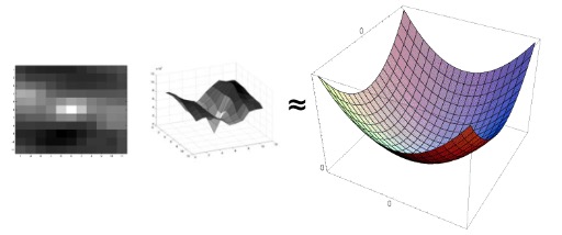
We can approximate $E(u,v)$ locally by a quadratic surface, and look for that instead.

Taylor Series Expansion

A function $f$ can be represented by an infinite series of its derivatives at a single point $a$.

$$ f = f(a)+\frac{f^{\prime}(a)}{1 !}(x-a)+\frac{f^{\prime \prime}(a)}{2 !}(x-a)^{2}+\frac{f^{\prime \prime \prime}(a)}{3 !}(x-a)^{3}+\cdots $$

Local Quadratic Approximation

Local quadratic approximation of $E(u,v)$ in the neighborhood of $(0,0)$ is given by the second-order Taylor expansion.

This could be simplified as the following equation, where $M$ is a structure tensor computed from image derivatives.

Interpreting the Second Moment Matrix

• $M$ is symmetric around the diagonal
  • Symmetric matrices have orthogonal eigenvectors
• $M$ is square
  • Square matrices are diagonalizable if some matrix $R$ exists such that $M = R^{-1}AR$ where $A$ has only diagonal entries and $R$ represents a change of basis (in 2D, a rotation).

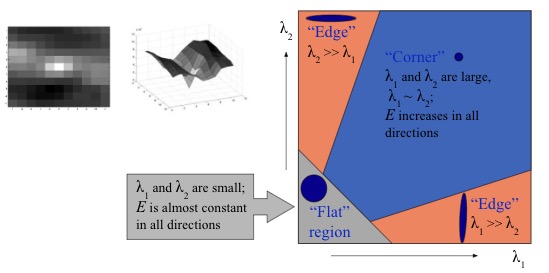
We want to decompose $M$ to be able to analyze the scale of these quadratic surfaces while ignoring the rotation. This means we care that it is a corner or an edge, not which rotation of edge.

Or we can combine $\lambda _1$, $\lambda _2$ with some constant $\alpha$ to computer the cornerness score:

$$ C={\lambda _1}{\lambda _2}-{\alpha}({\lambda _1}+{\lambda _2})^{2} $$

In linear algebra, for diagonal matrices,

• Determinant of a diagonal matrix is also the product of its diagonal entries
• Trace is just the sum of its diagonal entries

Therefore, we can avoid explicit eigenvalue computation by $$C=\operatorname{det}(A)-\alpha \operatorname{trace}(A)^{2}$$

Since $S^{-1}$ is the inverse matrix of $S$, we have $S^{-1}\cdot S = I$

$$\operatorname{det}(I) = \operatorname{det}(S\cdot S^{-1}) = \operatorname{det}(S)\cdot \operatorname{det}(S) = 1$$

We can now obtain that $\operatorname{det}(M) = \operatorname{det}(A)$

Thus,

$$C=\operatorname{det}(M)-\alpha \operatorname{trace}(M)^{2}$$

Harris Corner Detector

• Input image: computer $M$ at each pixel level
• Compute image derivatives $I_{x}$, $I_{y}$
• Compute $M$ components as squares of derivatives $I_{x}^{2}$, $I_{y}^{2}$
• Gaussian filter $g$ with width $s$: $g\left(I_{x}^{2}\right)$, $g\left(I_{y}^{2}\right)$, $g\left(I_{x} \circ I_{y}\right)$
• Compute cornerness $C=g\left(I_{x}^{2}\right) \circ g\left(I_{y}^{2}\right)-g\left(I_{x} \circ I_{y}\right)^{2} -\alpha\left[g\left(I_{x}^{2}\right)+g\left(I_{y}^{2}\right)\right]^{2}$
• Threshold $C$ to pick high cornerness
• Non-maximal suppression to pick peaks

Note: $a \circ b$ is Hadamard product (element-wise multiplication).

Scale Invariant Detection

Invariance & Covariance

Invariance: image is transformed and corner locations do not change.

Covariance / Equivariance: if we have two transformed versions of the same image, features should be detected in corresponding locations.

Properties of Harris Detector

• Corner response is invariant to image rotation
  • Ellipse rotates but its shape (i.e. eigenvalues) remains the same
• Partial invariance to affine intensity change
  • Invariance to intensity shift $I \rightarrow I + b$
  • Still affected by intensity scaling $I \rightarrow aI$
• Non-invariant to image scale

Automatic Scale Selection

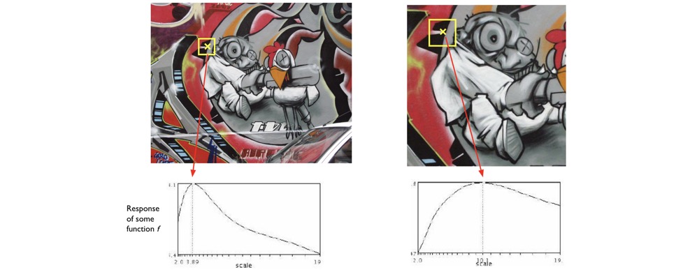
For a point in one image, we can consider it as a function of region size

For both image, we want to chose a scale that corresponds to the peak in both images. It’s likely that the peaks is the best scale for finding the correpsondences.