Authored by Tony Feng
Created on Jan. 17th, 2022
Last Modified on Jan. 17th, 2022
Intro
This sereis of posts contains notes from the course Self-Driving Fundamentals: Featuring Apollo published by Udacity & Baidu Apollo. This course aims to deliver key parts of self-driving cars, including HD Map, localization, perception, prediction, planning and control. I posted these “notes” (what I’ve learnt) for study and review only.
Intro to Control
Control is a strategy of actuating the vehicle to move it towards the road. For a car, the basic control inputs are steering, acceleration and break. The car uses controller inputs to minimize the deviation from the planning and maximize the passenger comfort.
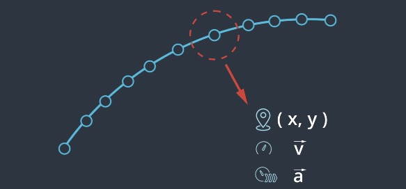
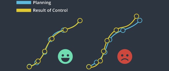
The controller receives trajectory as a sequence of way points. We use control inputs to move the vehicle towards those way points. The result of control should be as close as possible to the target trajectory.
- Controller needs to be accurate.
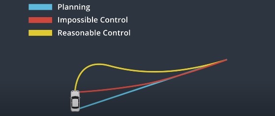
- The control strategy should be favaroble to vehicles.
- Actuation should be continuous to make the driving smooth.
Control Pipeline
There are two inputs of controller aspects: target trajectory and vehicle states. We use these 2 inputs to calculate the deviation between real trajectory and target trajectory.
The outputs of the controller are the values for the control inputs: steering, acceleration, and break. They are used to correct the deviation from the target trajectory.
Target Trajectory
It comes from the planning module. Each way point is designated a position and a reference velocity. The trajectory is updated at every timestamp.
Vehicle State
It is provided by the localization module. It includes the position of the vehicle. Also, it also includes data from internal sensors, such as speed, steering, and acceleration.
PID
Term P
The P controller will pull the vehicle back to the target trajectory as soon as it starts to deviate. Proportional means that the further the vehicle deviates, the harder the controller will steer back toward the target trajectory.
$$a=-K_{P} e$$
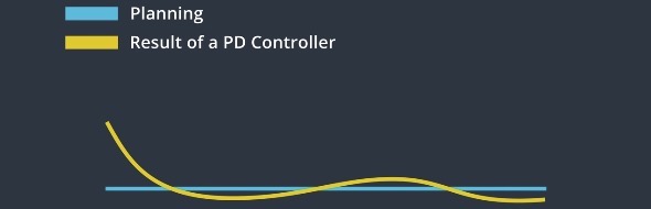
Term D
One problem of P controller is that it’s easy to overshoot the reference trajectory. We need the controller to be steadier when the vehicle is closer to the reference trajectory.
The D term of the PID steadies its motion. The PD controller has a damping term that minimizes how quickly the controller output changes.
$$a=-K_{P} e-K_{D} \frac{d e}{d t}$$
Term I
The I term is responsible for correcting any systemic bias of the vehicle. For example, the steering might be out of alignment, which would result in a constant steering offset. In that case, we need to steer a little bit to the side just to keep going straight. To handle this problem, the I controller penalilizes the accumulated error of the system.
$$a=-K_{P} e-K_{I} \int e d t-K_{D} \frac{d e}{d t}$$

Pros & Cons
Pros
- Proportional-Integral-Derivative Control (PID) only needs to know how far we have deviated from the target trajectory.
Cons
- PID is a linear algorithm, so it is not able to deal with complex problems. In real life, a self-driving car requires multiple PIDs, which means it’s hard to combine a latitudinal and longitudinal control.
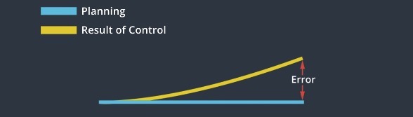
- Another problem is that it depends on real-time error measurement. Measurement delays can compromise the performance.
LQR
Model
Linear Qudratic Regulator is a model-based controller that uses the state of the vehicle to minimize error.
Apollo uses LQR for lateral control, which contains 4 conponents:
- The lateral error
- The rate of the change of lateral error (derivative)
- The heading error
- The rate of the change of the heading error (derivative))
$$ x=\left[\begin{array}{c} c t e \ c \dot{t} e \ \theta \ \dot{\theta} \end{array}\right] $$
$$ u=\left[\begin{array}{c} \text { steering } \ \text { acceleration } \ \text { brake } \end{array}\right] $$
This model can be represented by a State-space Equation:
$$ \dot{x} = Ax + Bu $$
, where $\dot{x} $ vector is the rate of change of the $x$ vector, so each component of $\dot{x} $ is just the derivative of the corresponding component of $x$. The equation captures how the change in state. Here you can find the implementation of LQR in Python
Term L
The equation is linear. When we there is a change to $x$ and $u$,
$$ \dot{x}+\Delta \dot{x}=A(x+\Delta x)+B(u+\Delta u) $$
the change to $\dot{x} $ will also satisfy this equation.
$$ \Delta \dot{x}=A \Delta x+B \Delta u $$
Term Q
We want to apply as few control inputs as possible to decrease overhead. In order to minimize these factors, we can keep running summation of errors and summation of control inputs.
E.g. When the car turns too far to the right, we add that error to the sum. When the control input steers the car back to the left, we subtract a bit from the control input sum. However, this approach causes problems. The positive errors to the right simply cancel out the negative errors to the left. The same would be true for control inputs.
Instead, we can multiply $x$ and $u$ by themselves, so the negative values will produce positive squares. They are called quadratic terms. We assign weights to these terms and the optimal $u$ should minimize summation overtime.
$$ w_{1} c t e^{2}+w_{2} c \dot{t e} e^{2}+w_{3} \theta^{2}+w_{4} \dot{\theta}^{2}+\ldots $$
Mathematically, they are defined using a cost function:
$$ \text { cost }=\int_{0}^{\infty}\left(x^{T} Q x+u^{T} R u\right) d t $$
, where $Q$ and $R$ represents a collection of weights for $x$ and $u$.
To minimize this cost function, one solution provided by Apollo is using a complicated scheme $K$, which can obtain $u$ through $x$.
$$ u = -Kx$$
So, finding an optimal $u$ is finding an optimal $K$. Many tools have access to solve $K$, once you provide $A$, $B$, $Q$, $R$.
MPC
Model Predictive Control heavily relies on mathematical optimzation. It’s a repeating process. It looks into the future to calculate and optimize a sequence of control inputs.
General Steps
- Building a model of the vehicle
- Using an optimization engine to calculate control inputs over a finite time horizon
- Implementing the first set of control inputs in the sequence
- Repeating the cycle
Why only to carry out the first set of control inputs?
Our measurements and calculation are only approximate. If we were to implement the entire sequence, the actual resulting vehicle state would diverge sharply from our model. We are better off continuously re-evaluating the optimal sequence of control inputs at every timestamp.
Defining Vehicle Model
This model approximates the physics of our car. It will model what will happen after we apply a set of control inputs to the vehicle.
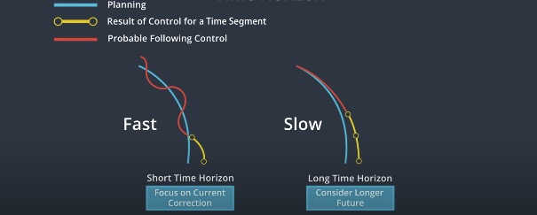
Time Horizon
We decide how far into the future we want MPC to look. However, there is a trade-off between the accruracy and how quickly we need to get a result.
- The further we look, more accurate our controller will be.
- The faster we get the result, the faster we can update the control inputs to the actual vehicle.
Optimization
We send the model to an optimization engine to search for the best control inputs among a dense mathemetical space.
Since our goal is to find a suitable control sequence, considering constraints can narrow the scope of our consideration and speed up the execution of the algorithm.
- Steering range that vehicle can achieve
- Acceleration range that can be used for acceleration/deceleration.
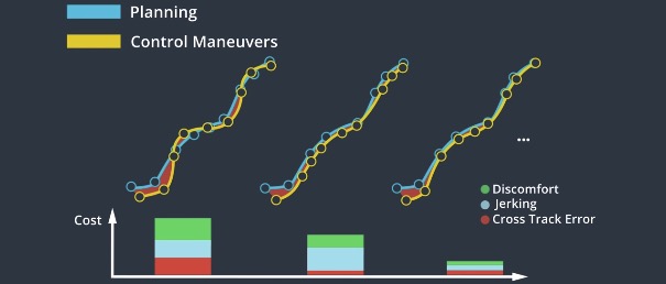
The optimization engine evaluates control inputs indirectly by modelling a trajectory for the vehicle. It uses a cost function which considers deviation from the target trajectory, acceleration, passenger comfort, etc.
Pros & Cons
Pros
- More accurate than PID contorl
- Works for different situations by using different cost functions
Cons
- More complex, slowere and harder to implement than PID control