Authored by Tony Feng

Created on Jan. 14th, 2022

Last Modified on Jan. 14th, 2022

Intro

This sereis of posts contains notes from the course Self-Driving Fundamentals: Featuring Apollo published by Udacity & Baidu Apollo. This course aims to deliver key parts of self-driving cars, including HD Map, localization, perception, prediction, planning and control. I posted these “notes” (what I’ve learnt) for study and review only.

Intro to Planning

In planning, we incorporate HD maps, localization, and prediction to build a trajectory for the vehicle.

The first step of planning is route navigation, which focuses on how to go from A to B on the map. Routing takes the map data as input and output a navigation path.

Once we have constructed a high-level route, we zoom into trajectory planning. It is about how to make subtle decisons to avoid obstacles and create a smooth ride for passengers.

The goal of trajectory planning is to generate a collision-free and comfortable trajectory to execute. This trajectory is defined by a sequence of points, each of which has an associated velocity and a timestamp to indicates when we should arrive at that point.

Routing

The goal of routing is to find the best path to travel from A to B on the map. It takes 3 input:

• The map
  • Road network
  • Real-time traffic info
• Our current position on the map
• The destination

World to Graph

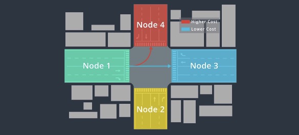
Apollo uses searching algorithms to find a route. Before that, the system reformats the map into a graph, where the nodes represent the sections of road and edges represent connections between those sections.

A* and Grid World

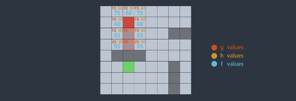
First, we calculate the cost it takes to travel from the start node to that candidate node. ($g$ -> candidate cost)

Second, we estimate how much it costs to travel from that candidate node to the goal. ($h$ -> estimated cost / heuristic cost)

The best candidate node is the node that has the minimum cost $f = g + h$.

The cost may vary based on the real-time traffic info.

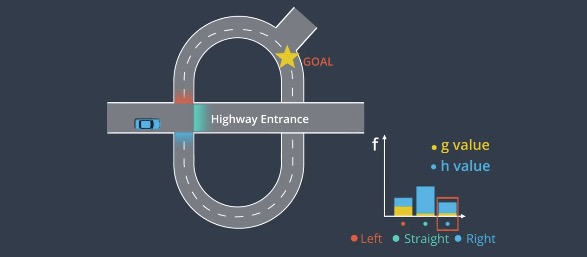
For example, it takes a lot of effort to turn through the intersection, so we assign a higher $g$ value to the node indicating turning left.

For the highway option, we realize that we may have to travel a long way to exit the highway and return back to reach the goal. So we assign higher $h$ value to this node.

Trajectory Generation

The high-level map route is only part of the planning process. We still need to build low-level trajectories to deal with objects, like bicycles, pedestrians, that aren’t part to the map. This scenario requires lower-level, high-precision planning.

Frenet Coordinates

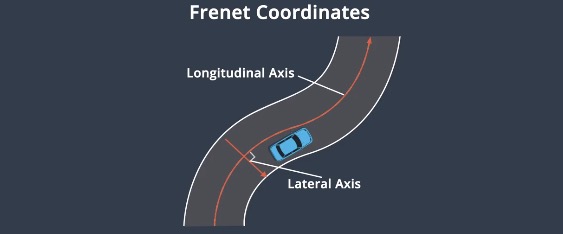
Tradionally, we describe the position of an object using Cartesian coordinates, but it is not optimal for vehicles. If we don’t know the road, we don’t know how far the vehicle has traveled or whether it is deviated from the center of the lane.

Frenet coordinate describes the position of the car with respect to the road. Longitudinal axis represents the distance along the road, while lateral axis represents the displacement from the longitudinal line. These two axis are perpendicular.

3D Trajectory

The goal is to generate a trajectory defined by a series of points. We can fit a curve to these points to create a geometric representation of the trajectory.

Since moving obstacles may block parts of the road temporarily, each points has a timestamp. We can combine the timestamp with the output of the prediction module to verify if the points are vacant at the time we plan to move through them.

These timestamps create a 3D trajectory with each point defined by a 2D space and a third dimension in time.

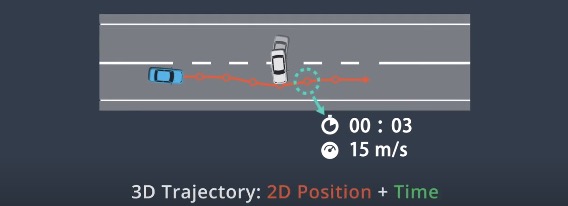
We also designate a velocity for each point, which ensures that the vehicle can reach the point on schedule.

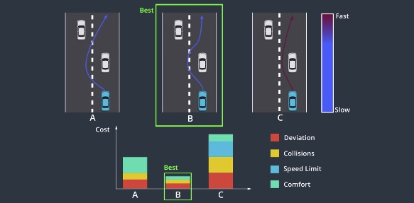
Evaluating a Trajectory

Constraints

• The final position aligns with the center line of the lane.
• The distance from obstacles at every point of the trajectory
• Traffic laws, such as speed limit, etc.
• The trajectory should be physically viable for the vehicle.
• Passenger’s comfort

Cost Function We can use cost function to choose a right trajectory among different possible candidates. Different scenarios require different cost functions.

EM Planning

EM Planning is also called Path-Velocity Decoupled Planning

Path Planning

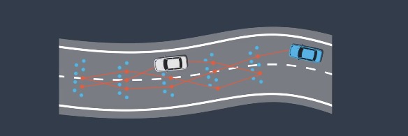
• Generating candidate paths
  • Segmenting the road into cells
  • Randomly sampling the points from each cell
  • Selecting one point from each cell and connecting points together
• Using a cost function which considers smoothness, safety, and other factors
• Ranking the paths based on their costs and choose a best path

Speed Planning

• Determining a sequence of speeds (a speed profile) associated with points
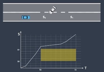
• Using ST Graph can help design and select the speed profile
  • S represents the longitudinal displacement of the vehicle
  • T represents the time
• Discretizing the ST graph into multiple cells
  • Speed changes between cells
  • Speed remains constant with each cell
  • Obstacles can be drawn as rectangles that block off certain parts of the road during certain time periods
• Optimizing the speed profile subject to various constraints

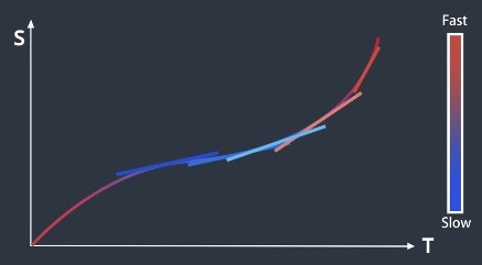
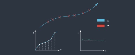
Trajectory Optimization

Discretization makes problems easier to solve, but the solution are not smooth. We can quadratic programming to convert discrete solutions into a smooth trajectory, which fits a smooth non-linear curve to these piecewise linear segments.

Lattice Planning

3D Trajectory $\rightarrow$ Longitudinal Dimension + Lateral Dimension + Time Dimension

We can convert it into 2D problems

• ST Trajectory: Longitudinal Dimension + Time Dimension
• SL Trajectory: Longitudinal Dimension + Lateral Dimension

Since the problems share the same Longitudinal Dimension, we can use it to transform them back to the Cartesian coordinate frame and combine them to construct a 3D trajectory.

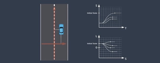
Steps

• We start by projecting the vehicle’s initial state onto ST and SL frames.
• We select ending state by sampling multiple candidate ending states from pre-selected patterns.
• For each candidate ending state, we build a set of trajectories to transition our vehicle from its inital state to the ending state.
• We use cost function to select an optimal trajectory.

Ending States for ST

• Cruising
• Following
• Stopping

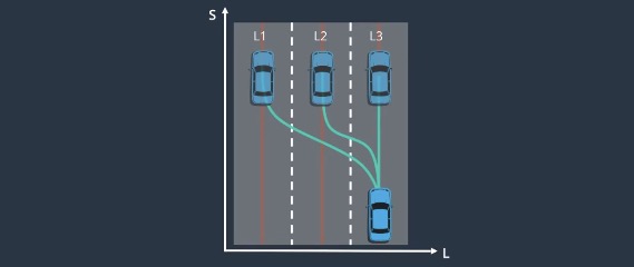
Ending States for SL

We assume that the vehicle will steadily align with the central line of the lane no matter what ending state it would enter. The trajectory should end with the vehicle aligned with the lane and driving straight.

Polynomial Fitting

We will fit a polynomial to the initial state and the ending state.

Here, the initial conditions and end conditions are both tuples with position, speed, and acceleration on $s$ coordinate. Note that speed is the first-order derivative of position and acceleration is the second-order derivative of position.

Usually, we denote the derivative with respect to time as a dot above a variable.

• Initial condition: $(s_{0}, \dot{s_0}, \ddot{s_0})$
• Ending condition: $(s_{1}, \dot{s_1}, \ddot{s_1})$

The polynomial we are going to fit looks like:

$$s(t)=a t^{5}+b t^{4}+c t^{3}+d t^{2}+e t+f$$

By taking the derivative of this form we get:

$$\dot{s(t)}=5 a t^{4}+4 b t^{3}+3 c t^{2}+2 d t+e$$ $$\ddot{s(t)}=20 a t^{3}+12 b t^{2}+6 c t+2 d$$

Now we plug in the initial condition and ending condition, we have 6 equations. Here we suppose the ending condition happen at time $t = T$.

$$s_{0}=f$$ $$\dot{s_0}=e$$ $$\ddot{s_0}=2d$$ $$s_{1}=a T^{5}+b T^{4}+c T^{3}+d T^{2}+eT+f$$ $$\dot{s_{1}}=5 a T^{4}+4 b T^{3}+3 c T^{2}+2 d T+e$$ $$\ddot{s_{1}}=20 a T^{3}+12 b T^{2}+6 c T+2 d$$

With these equations, we can solve for $a$, $b$, $c$, $d$, $e$, and $f$. This represents a curve that smoothly connects two conditions.