Authored by Tony Feng

Created on Oct 4th, 2022

Last Modified on Oct 4th, 2022

Intro

This sereis of posts contains a summary of materials and readings from the course CSCI 1460 Computational Linguistics that I’ve taken @ Brown University. The class aims to explore techniques regarding recent advances in NLP with deep learning. I posted these “Notes” (what I’ve learnt) for study and review only.

Theories of Word Meaning

The Meaning of a word

Naive BOW model has no notion of word meaning (e.g. “cat” and “kitten” shoud have similar meanings, but it treats them as different words). Here comes to a problem: How to set boundaries to define words?

• Words refer to sets
• Words refer to things
• Words refer to concepts
• Words are defined by the context

The Distributional Hypothesis

The meaning of a word is defined by its context, and this leads to another question: What is context?

• Perceptional context / Linguistic context
• Symbolic features / Real-valued “impressions”
• First order associations / Higher-order abstraction

The distributional hypothesis is that words found in the same contexts usually have similar meanings. It is clear how words are “learned” according to the theory and the model correlates well with lots of data on humans. However, it is “holostic”, because the meaning is always changing based on different contextss.

Vector Space Models

Definition

Words are represented as vectors, and those have similar meanings are nearby in the space.

Term-document Matrix

• word meaning = set of documents in which it occurs
• It can be binary indicators, real value counts, tf-idf values, etc.
• It captures broad topical-similarity and co-occurrence, rather than the “same meaning”.
• It is good for document classification tasks, retrieval.

Word-Context Matrix

• It finds all sentences containing that word.
• It can be binary indicators, real value counts, tf-idf values, etc.
• The similar words don’t necessarily co-occur, but they occur in similar contexts.
• It captures more grammatical similarity and lexical similarity.

Computing Similarity

Extract Equivalence

• w1 == w2 iff their vector representations are identical
• However, the language is too varaible and this would never work

Jaccard Similarity

• $S= \frac{intersection(v_1, v_2)}{union(v_1, v_2)} $
• It works well for binary vectos, but needs adjustments for real-valued dimensions.

Euclidean Distance

• $E = \sqrt{\sum_{i=0}^{n}\left(v_{1}^{i}-v_{2}^{i}\right)^{2}} $
• It assumes similar words will be of similar magnitude (i.e., occur with similar frequency).

Cosine Similarity

• $C = \frac{\overrightarrow{v 1} \cdot \overrightarrow{v 2}}{|\overrightarrow{v 1}||\overrightarrow{v 2}|} = \frac{\sum_{i=0}^{n} v_{1}^{i} v_{2}^{i}}{\sqrt{\sum_{i=0}^{n} (v_{1}^{i})^{2}} \sqrt{\sum_{i=0}^{n} (v_{2}^{i})^{2}}}$
• Dot product (scalar product / inner product) of two words vectors
• It can be explained as projection of v1 onto v2
• v1·v2 == 0 if vectos are orthogonal
• v1·v2 == -1 if they have opposite directions
• v1·v2 == 1 if they are parallel

Word Embeddings

Word Vectors vs. Embeddings

Word Vectors: sparse, very high-dimensional
Word Embeddings: dense, low dimensional, dimensions are not directly interpretable

Why Word Embeddings?

• Lower dimensional = less computationally intensive
• Lower dimensional forces abstraction
• Lower dimensional removes noise:
• Dimensionality reduction can capture “second order” effects (E.g., w1 occurs with c1, w2 occurs with c2, c1 and c2 are similar. Thus, w1 and w2 are similar.)

We can use Dimensionality Reduction to get them: 1) Matrix Factorization, 2) Neural Networks.

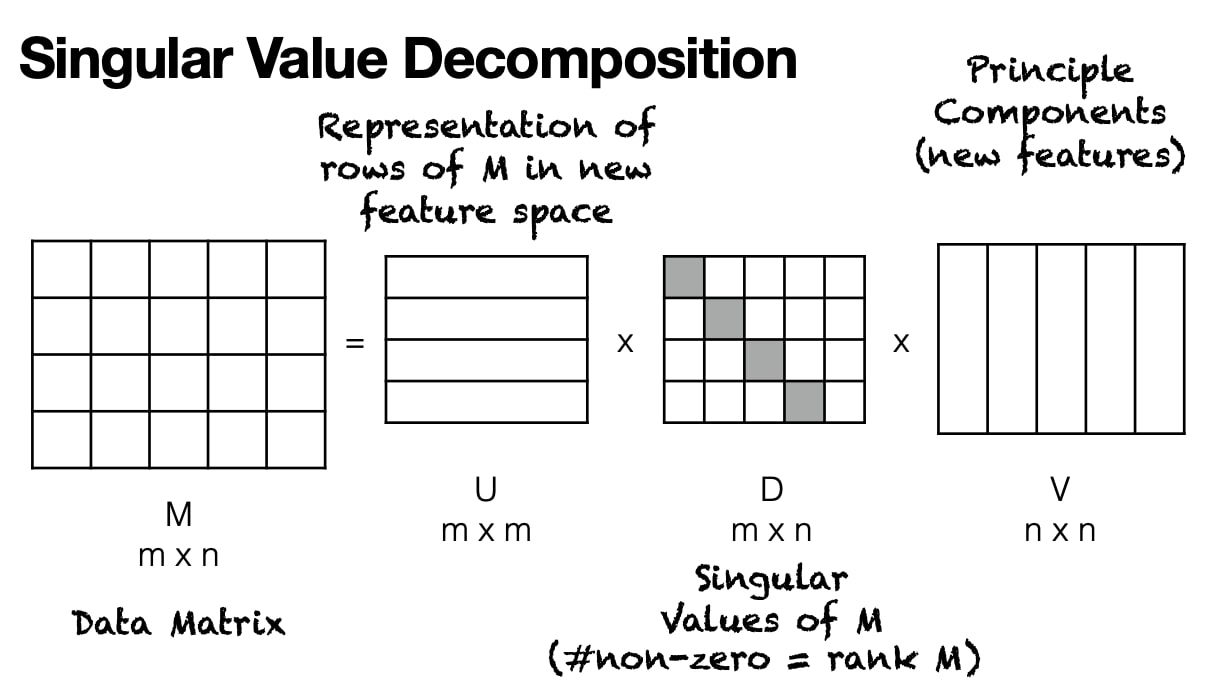
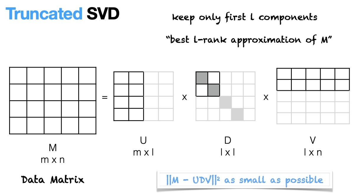
Dimensionality Reduction

It represents the data points in a new feature space by transforming the feature matrix. The new feature space is more informative for ML but is less interpretable to humans.

Principle Component Analysis (PCA) Low Rank Assumptioin: we typically assume that our features contain a large amount of redundant information.
M = U * D * V, where U contains word embeddings.

For more info, please read this article: Principal Component Analysis in Machine Learning