Authored by Tony Feng

Created on Feb 14th, 2022

Last Modified on Feb 14th, 2022

Intro

This sereis of posts contains a summary of materials and readings from the course CSCI 1430 Computer Vision that I’ve taken @ Brown University. This course covers the topics of fundamentals of image formation, camera imaging geometry, feature detection and matching, stereo, motion estimation and tracking, image classification, scene understanding, and deep learning with neural networks. I posted these “Notes” (what I’ve learnt) for study and review only.

Local Feature Description

Before we’re able to start matching points in images, we must first find a way to meaningfully describe each key point. Harris Corners only tell us where the key points are and not what information exists at those points

Possible Feature Descriptors

• Templates
  • Intensity, gradients, or other self-defined features
• Histograms
  • Color, texture, SIFT descriptors, etc.

Histograms

A histogram is a plot where the x axis corresponds to pixel values (0-255 for 8-bit encoding), and the y axis measures to the frequency of pixels with values corresponding to the x-axis.

e.g. at an intensity of 50, we see that there are around 5500 pixels in the image with that intensity).

Scale Invariant Feature Transform

SIFT: At a high level, we want to compute a histogram around each key point using local information.

Algorithm

• Find Harris corners scale-space extrema as feature point locations
• Corner post-processing
  • Subpixel position interpolation
  • Discard low-contrast points
  • Eliminate points along edges
• Orientation estimation per feature point
• Descriptor extraction

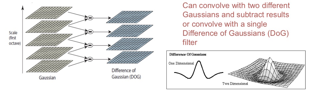
Scale-space Extrema

• Find points whose surrounding patches (at some scale) are distinctive
• Apply convolution with a Gaussian mask gives some idea of what is going on around a pixel
• Gaussian masks have a natural scale - their standard deviation
  • Difference of Gaussians

• Automatic Scale Selection
• Normalize the patch to fix size

Orientation Estimation

Gradient Orientation Histogram

To build this histogram, we bin the possible range of gradient orientations/directions (0 to 2pi radians) into a discrete number of bins (8 here) and, for each bin, we count the number of gradients that have those corresponding orientations.

Dominant Orientation $\theta$

We also compute an average gradient direction (black vector) of all the gradients in the local window; this is the dominant orientation of this neighborhood.

Orientation Normalization

We then rotate each region’s gradients so that all dominant gradient orientations point in the same direction (e.g. up). This will affect the orientation histogram by shifting the plot. We do this because we want the key point features to be invariant to rotation.

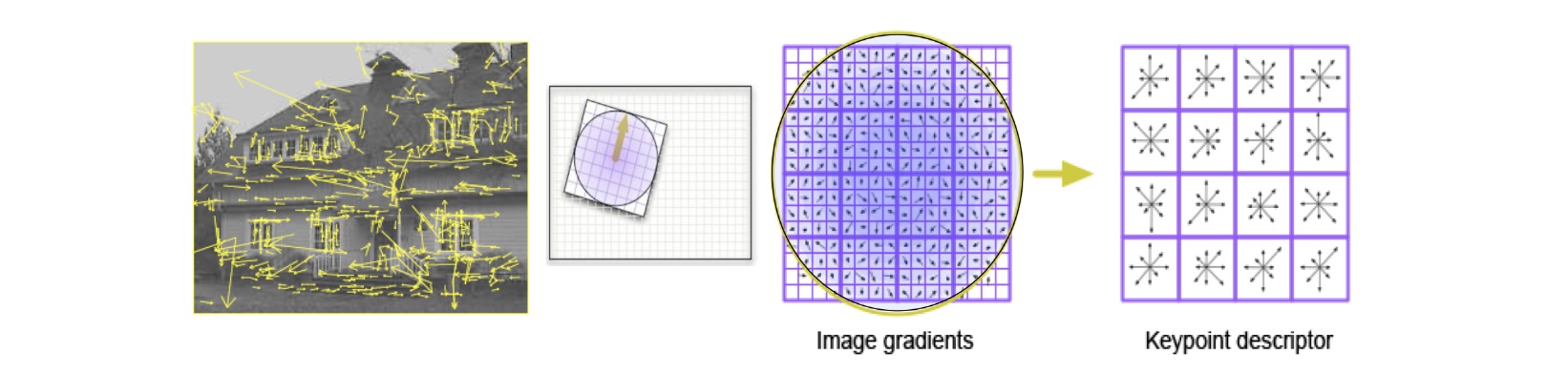
Keypoint Descriptor

A 16x16 neighbourhood around the keypoint is taken. It is divided into 16 sub-blocks of 4x4 size.

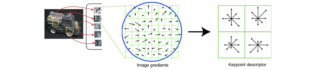
For each sub-block, 8 bin orientation histogram is created. So a total of 128 bin values are available.

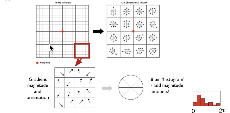
It is represented as a vector to form keypoint descriptor. (16 cells * 8 orientations = 128 dimensional descriptor)

In addition to this, several measures are taken to achieve robustness against illumination changes, etc.

• One trick we can employ to reduce the contribution of pixels farther from the keypoint is to apply a Gaussian filter over the entire 16x16 window.
• Clamp all vector values > 0.2 to 0.2
• Renormalization

Feature Matching

Basic Idea

It generally refers to computing distance between feature vectors to find correspondence.

• Euclidean Distance
• Cosine Similarity

Problems

• Threshold is hard to pick.
• Non-distinctive features could have lots of close matches, only one of which is correct.

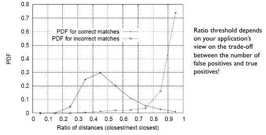
NN Distance Ratio

Here, we introduce the approach by comparing distances of 2 nearest feature vector neighbor.

• If $d_1 \approx d_2$, ratio $\frac{d_1}{d_2}$. (too close)
• AS $d_1 \ll d_2$, ratio $\frac{d_1}{d_2}$ tends to 0

Too choose the ratio, we can compute a probability distribution functions of ratios based on keypoints with hand-labeled ground truth.

Other Local Descriptors

• SURF
• Shape Context
• Self-similarity Descriptor