Authored by Tony Feng

Created on Jan 31st, 2022

Last Modified on Feb 2nd, 2022

Intro

This sereis of posts contains a summary of materials and readings from the course CSCI 1430 Computer Vision that I’ve taken @ Brown University. This course covers the topics of fundamentals of image formation, camera imaging geometry, feature detection and matching, stereo, motion estimation and tracking, image classification, scene understanding, and deep learning with neural networks. I posted these “Notes” (what I’ve learnt) for study and review only.

Filtering

Def

An operation that modifies a (measured) signal, which includes:

• removing undesirable components
• transforming signal in a desirable way
• extract specific components of a signal.

We are interested in measured or discrete signals because that is what we get from hardware such as sensors.

1D Filtering: Moving Average

We have a signal $S \in \mathcal{R}^{m \times 1}$, where $m$ is the number of samples we take of the signal, and each sample is a single scalar value. The moving average $h[n]$ at the point $n$ is the average value of the signal over the $k$ most recent samples, which can be represented as:

$$h[n]=\frac{1}{k} \sum_{i=n-k+1}^{n} S[i]$$

or $$h[n]=\frac{1}{k} {I}^{T} S[n-k+1: n]$$

, where $I$ is and identity vector.

2D Filtering

For images, we’re interested in filtering along two spatial axes ($x$ and $y$) rather than a single one.

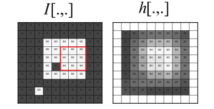
$$h[m, n]=\sum_{k, l} f[k, l] S[m+k, n+l]$$

The equation says that the filtered value at a location $(m,n)$ is the sum over products of the filtering function $f$ and the image $S$ in a local neighborhood. The size of the window is determined by $k$ and $l$.

Image Filtering

Box Filter/Mean Filter

The box filter blurs the image because for each pixel, the values of its neighbors is averaged with it, and preserve mean image intensity.

Gaussian Filter

The filter function is constructed by sampling the gaussian function at uniform intervals. It’s a linear filter.

Gaussian pdfs have infinite extent. Gaussian filters are discrete finite samplings of the Gaussian pdf. What that means is that the filter can be arbitrarily large, and it will never be zero (to numerical precision).

$$ G_{\sigma}=\frac{1}{2 \pi \sigma^{2}} e^{-\frac{\left(x^{2}+y^{2}\right)}{2 \sigma^{2}}} $$

Unlike box filter, does not result in ‘grid’-like artifacts.

Gaussian Filter Properties:

• Gaussian convolved with Gaussian is another Gaussian
• We can smooth with small-width kernel, repeat, and get same result as larger-width kernel
• Convolving twice with Gaussian kernel of width $\sigma$ is same as convolving once with kernel of width $\sigma \sqrt{2} $
• How big should the Gaussian filter be?
  • Values at edges should be near zero
  • Gaussians have infinite extent
  • Set filter half-width to about $3\sigma$

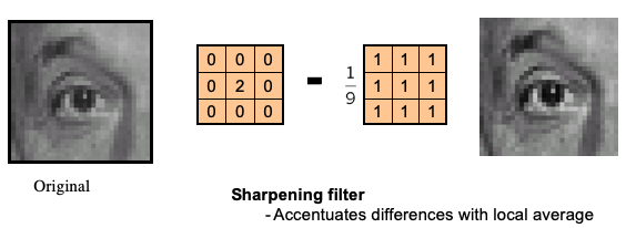
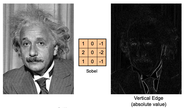
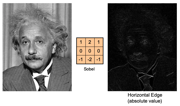
Sobel Filter

It has “1 2 1” pattern and is often used in edge detection. It works by calculating the gradient of image intensity at each pixel within the image. It’s a high pass filter.

Median Filter

It is a non-linear filter. It operates over a window by selecting the median intensity in the window. Median filtering is sorting.

It’s good at removing noises. If we increase the size of the window, it can maintain strong edges, while other parts become blurred.

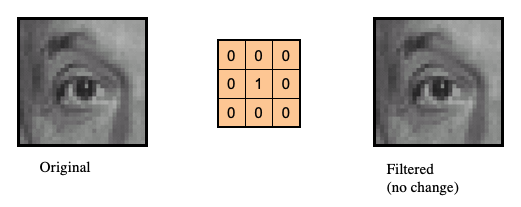
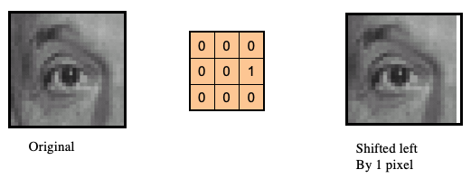
Practice with Linear Filters

We can use filter to

• Enhance images
  • Denoise, resize, increase contrast, etc.
• Extract information from images
  • Texture, edges, distinctive points, etc.
• Detect patterns
  • Template matching

Examples

Dealing with Borders

Pixels are undefined outside the border of our image, so to apply the filter near the boundary, we nee to extend the image past its boundary using one of many possible methods.

• Clip filter: any value outside of the image is set to 0
• Copy edge: copy the pixel value of the nearest edge
• Wrap around: copy the values near the opposite edge
• Reflect across edge: treat out-of-bounds regions as ‘mirrors’ that reflect near-surface image pixels in reverse order

Properties of Image Filtering Methods

Correlation and Convolution

2D Correlation

$$h[m, n]=\sum_{k, l} f[k, l] S[m+k, n+l]$$

2D Convolution

$$h[m, n]=\sum_{k, l} f[k, l] S[m-k, n-l]$$

Convolution is the same as correlation with a 180° rotated filter kernel.

Correlation and convolution are identical when the filter kernel is rotationally symmetric (a square matrix that is equal to its transpose).

For symmetric filters: use either convolution or correlation

For non-symmetric filters: correlation is template matching.

More can be found here

Linear Filter Properties

• Linearity means that filtering an image with two (different) filters $f1$ and $f2$ results in the same output as filtering the images separately first before summing the intermediate outputs. $$ imfilter(I, f1 + f2) = imfilter(I,f1) + imfilter(I,f2) $$
• Translation invariance means that shifting the original image before filtering results in the same output as filtering then shifting. $$imfilter(I,shift(f)) = shift(imfilter(I,f))$$
• Any linear, shift-invariant operator can be represented as a convolution.

Separability

We can use an outer product to decompose the 2D filter into two 1D filters, where one is represented as a row column and the other a row vector.

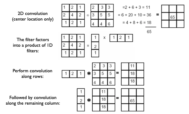
Note: Convolution vs filtering doesn’t matter here because the filter is symmetric.

Assume we have $M * N$ image, $P*Q$ filter

• 2D convolution: $MNPQ$ multiply-adds

• Separable 2D: $MN(P+Q)$ multiply-adds

Speed up = $\frac{PQ}{(P+Q)}$, e.g. 9*9 filter = 4.5 times faster

In Gaussian Filters, a 2D Gaussian can be expressed as the product of two functions, a function of $x$ and a function of $y$.

$$ G_{\sigma}=\frac{1}{2 \pi \sigma^{2}} e^{-\frac{\left(x^{2}+y^{2}\right)}{2 \sigma^{2}}} = \left(\frac{1}{2 \pi \sigma^{2}} e^{-\frac{x^{2}}{2 \sigma^{2}}}\right)\left(\frac{1}{2 \pi \sigma^{2}} e^{-\frac{y^{2}}{2 \sigma^{2}}}\right)$$

Applications of Filters

• Template matching (SSD or Normxcorr2)
  • SSD can be done with linear filters, is sensitive to overall intensity
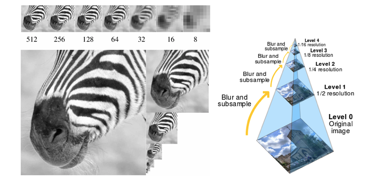
• Gaussian pyramid
  • Coarse-to-fine search, multi-scale detection
• Laplacian pyramid
  • Teases apart different frequency bands while keeping spatial information
  • Can be used for compositing in graphics
• Downsampling
  • Need to sufficiently low-pass before downsampling

Sampling

Image Pyramid

Aliasing

Aliasing occurs when we sample a signal at a frequency that is too low such that we can’t properly reconstruct the original signal. In the image below, black points are samples, but we may get a different-looking reconstruction.

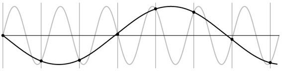
When two signals become indistinguishable from one another due to sampling, they are ‘aliases’ of one another.

In real world, temporal and spatial aliasing often happens when the sampling rate is not high enough.

Nyquist-Shannon Sampling Theorem

When sampling a signal at discrete intervals, the sampling frequency must be $\ge 2 f_{max}$, max frequency of the input signal, to guarantee a perfect reconstruction.

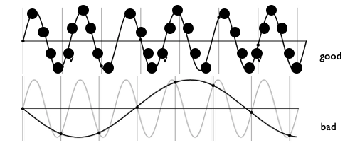
Anti-aliasing

• Sampling more often
• Removing all frequencies that are greater than half the new sampling frequency
  • Remove high frequencies with a low pass filter (e.g. Gaussian Filter)
  • It will lose info