Authored by Tony Feng
Created on Mar 7th, 2022
Last Modified on Mar 7th, 2022
Intro
This sereis of posts contains a summary of materials and readings from the course CSCI 1430 Computer Vision that I’ve taken @ Brown University. This course covers the topics of fundamentals of image formation, camera imaging geometry, feature detection and matching, stereo, motion estimation and tracking, image classification, scene understanding, and deep learning with neural networks. I posted these “Notes” (what I’ve learnt) for study and review only.
Stereo Pipeline
- Calibrating cameras
- Rectifying images (i.e. 8-point algorithm)
- Correspondence
- Estimate depth
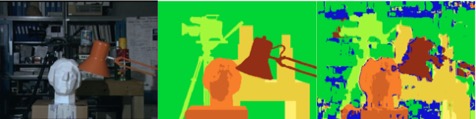
Correspondence here means dense correspondence, i.e. for each point on the left image we find its correspondence on the right.
Correspondence allows measurement of disparity: the difference in the image coordinates of the projections of a given world point into each camera.
Basic Stereo Matching
Algorithm
- Rectify the two stereo images to transform epipolar lines into scanlines
- For each pixel x in the first image
- Find the corresponding epipolar scanline in the right image
- Examine all pixels on the scanline and pick the best match $x'$
- Compute disparity $x - x’$ and set depth $ Z = f \frac{T}{x - x’}$
Effect of Window Size
When calculating SSD or Normalised Correlation of an image window is chosen around the point:
- Smaller window: more detail but more noise
- Larger window: Smoother disparity maps but less detail
Problems
- Window size is fixed across the image, but viewed objects differ in size and depth.
- Uniform regions always match.
- Values on dense disparity map are only reliable where there is some local variation in intensity e.g. near edges.
- Dense disparity is computationally expensive in spatial domain.
Stereo Constraints
So far, matches are independent for each point. What constraints or priors can we add?
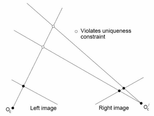
Uniqueness
For any point in one image, there should be at most one matching point in the other image

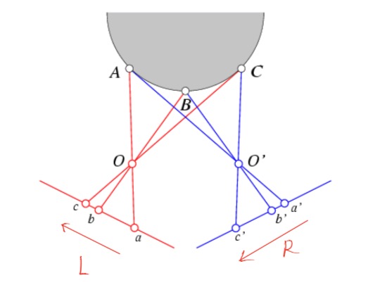
Ordering
Corresponding points should be in the same order in both views for most cases.
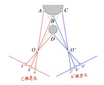
Ordering constraint doesn’t hold when occlusion occurs.
Smoothness
We expect disparity values to change slowly (for the most part).
Disparity Space Image
Idea
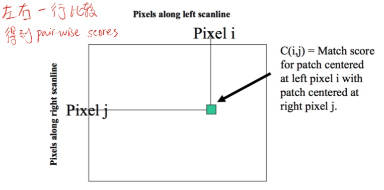
DSI for one row represents pairwise match scores between patches along that row in the left and right image.
DSI Formation
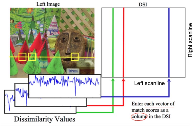
Goal
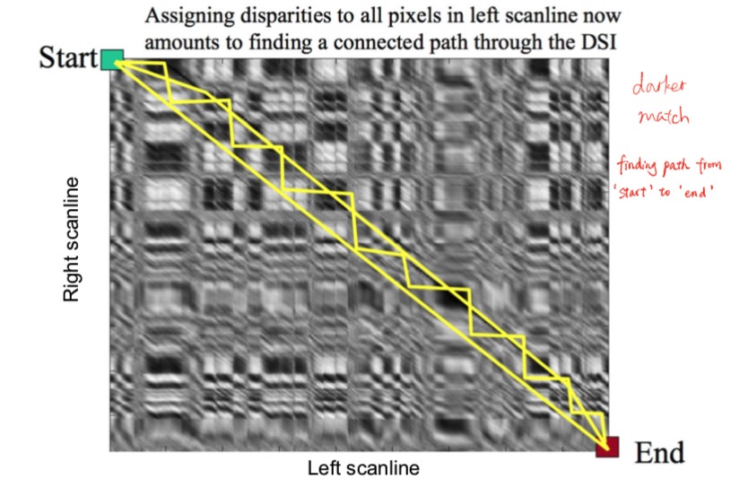
Assigning disparities to all pixels in the left scanline now amount to finding a connected path through DSI. We need to find the minimum cost path through the matrix of all pairwise matches between two corresponding rasters.
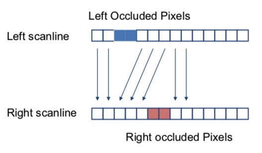
Correspondence Search
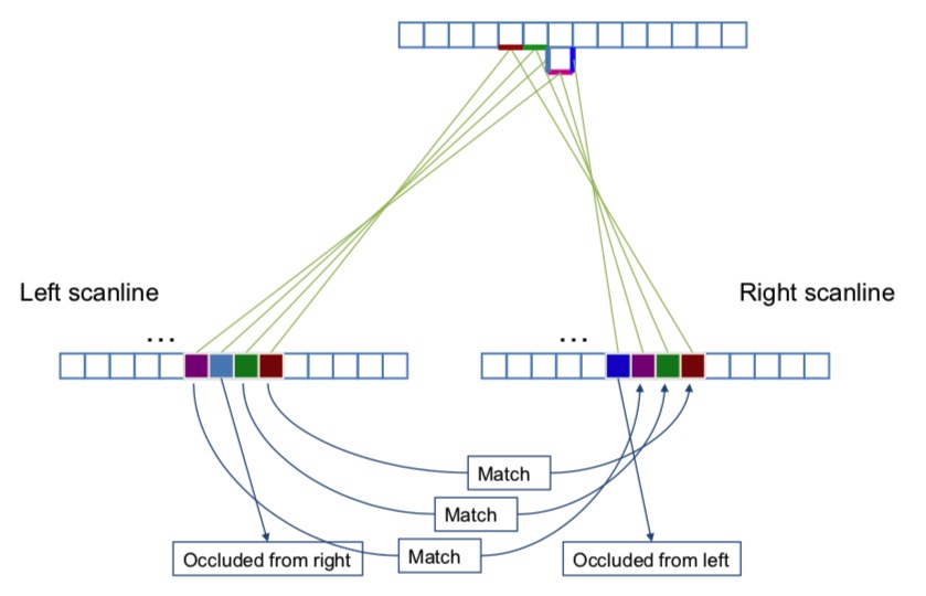
As we traverse the scanline there are 3 possibilities
- Pixels match, at a cost based on similarity
- Left occlusion, at a cost associated with an unmatched pixel
- Right occlusion, at a cost associated with an unmatched pixel
Assuming that row, column of DSI represents right and left image respectively.
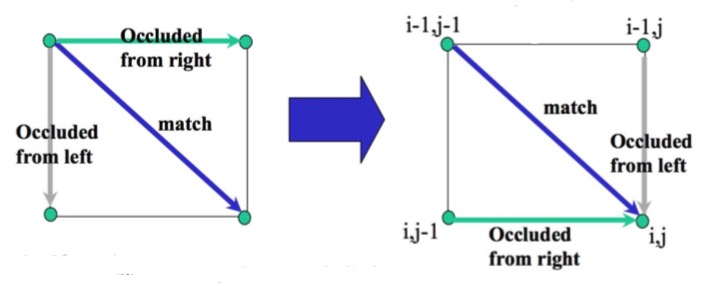
$$C(i, j) = \text{min}(C(i-1, j-1) + D(i, j), C(i-1, j) + OC, C(i, j-1) + OC) $$
, where $C$ means cost, $D$ means dissimilarity, $OC$ means occlusioin constant.
Performance
Strengths
- Produces good results in polynomial time
- Can deal with occlusions
Weaknesses
- Can be hard to find the right cost function
- Hard to enforce consistency between neighbouring rasters along vertical direction.
- Must enforce the ordering constraint