[Computer Vision] Stereo Vision

Authored by Tony Feng

Created on Feb 23th, 2022

Last Modified on Mar 7th, 2022

Intro

This sereis of posts contains a summary of materials and readings from the course CSCI 1430 Computer Vision that I’ve taken @ Brown University. This course covers the topics of fundamentals of image formation, camera imaging geometry, feature detection and matching, stereo, motion estimation and tracking, image classification, scene understanding, and deep learning with neural networks. I posted these “Notes” (what I’ve learnt) for study and review only.

Multi-view Geometry

Problems

Camera Motion
Stereo Correspondence
Structure from Motion
Optical Flow

General Pipeline

Calibrating cameras
Rectifying images
Correspondence
Estimate depth

Stereo Geometry

One case of 3D reconstruction is when we don’t know how far a 3D object is nor the shape of it. But we do know the camera geometry and the projection of that shape onto our images. Now, we’re trying to find what $X$ is.

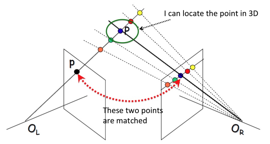
However, multiple points in 3D can result to the same projection!

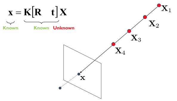
We need one point that is along the lines that is the true $(x, y)$ position. Triangulation uses two images and you try to find the same $x$ point in both images. Since both images represent the same object in space, they would both intersect at a point. The second camera/images fixes the image of $X$ along the line we see.

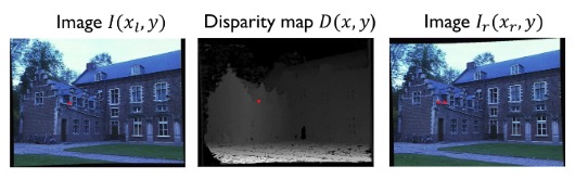
In the depth image, brighter means it’s closer to the camera, and darker means it’s farther to the camera.

Calibrated Stereo Case

Parallel Calibrated Cameras

$$ (x_r, y) = (x_l + D(x,y), y)$$

We assume that the two calibrated cameras (we know intrinsics and extrinsics) are parallel. The distance between the right camera and the left camera is called baseline.

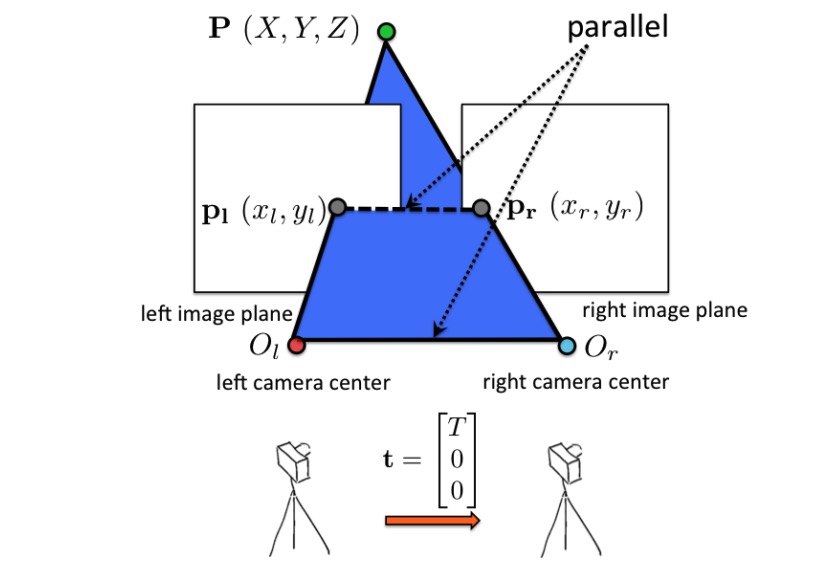
Since two images lie on the same plane, the lines $O_l O_r$ and $P_l P_r$ are parallel. Also, $O_l$ and $ O_r$ have the same $y$. This implies $y_l = y_r$

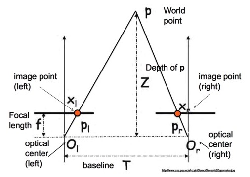
Depth is inversely proportional to disparity.

$$\frac{T}{Z} = \frac{T + x_r - x_l}{Z - f}$$

Scanline

For each point $P_l$, how do I get $P_r$? By matching. Patch around $P_l$ should look similar to the patch around $P_r$. We can scan the line and compare patches between two images.

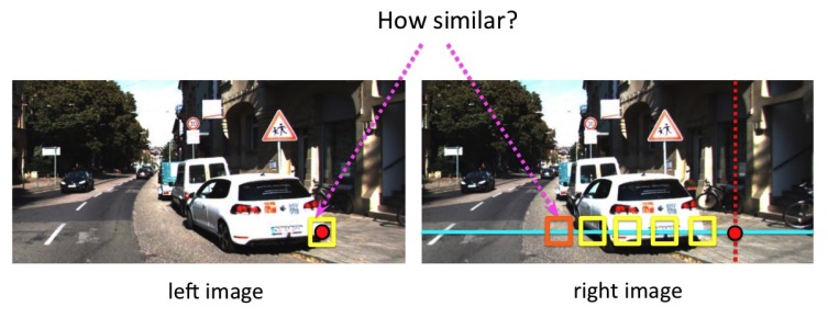
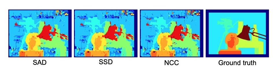
Matching Cost

Epipolar Geometry

Now, we consider it in a general case. The relationship between 2 camera pose is $\left [R | t \right ]$.

Epipolar Line and Epipole

All points from the projective line $O_l P_l$ project to a line on the right image plane. This time the line is not (necessarily) horizontal.

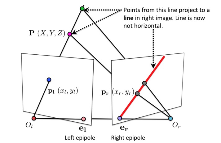
Points $O_l$, $O_r$ and a point $P$ in 3D lie on a plane. We call this the epipolar plane. This plane intersects each image plane in a line. We call these lines epipolar lines.

All epipolar lines are converged at a point of each image called epipole. Two camera centers and epipoles are on the same line.

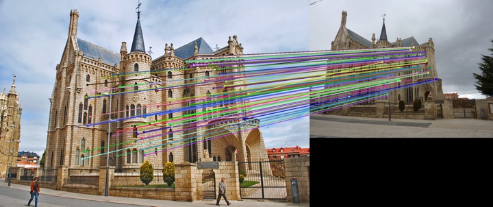
Epipolar geometry is useful because it constrains our search for the matches:

For each point $P_l$, we need to search for $P_r$ only on a epipolar line.
All matches lie on lines that intersect in epipoles.

Essential Matrix

The assumption is that points are aligned within camera coordinate axis (calibrated camera).

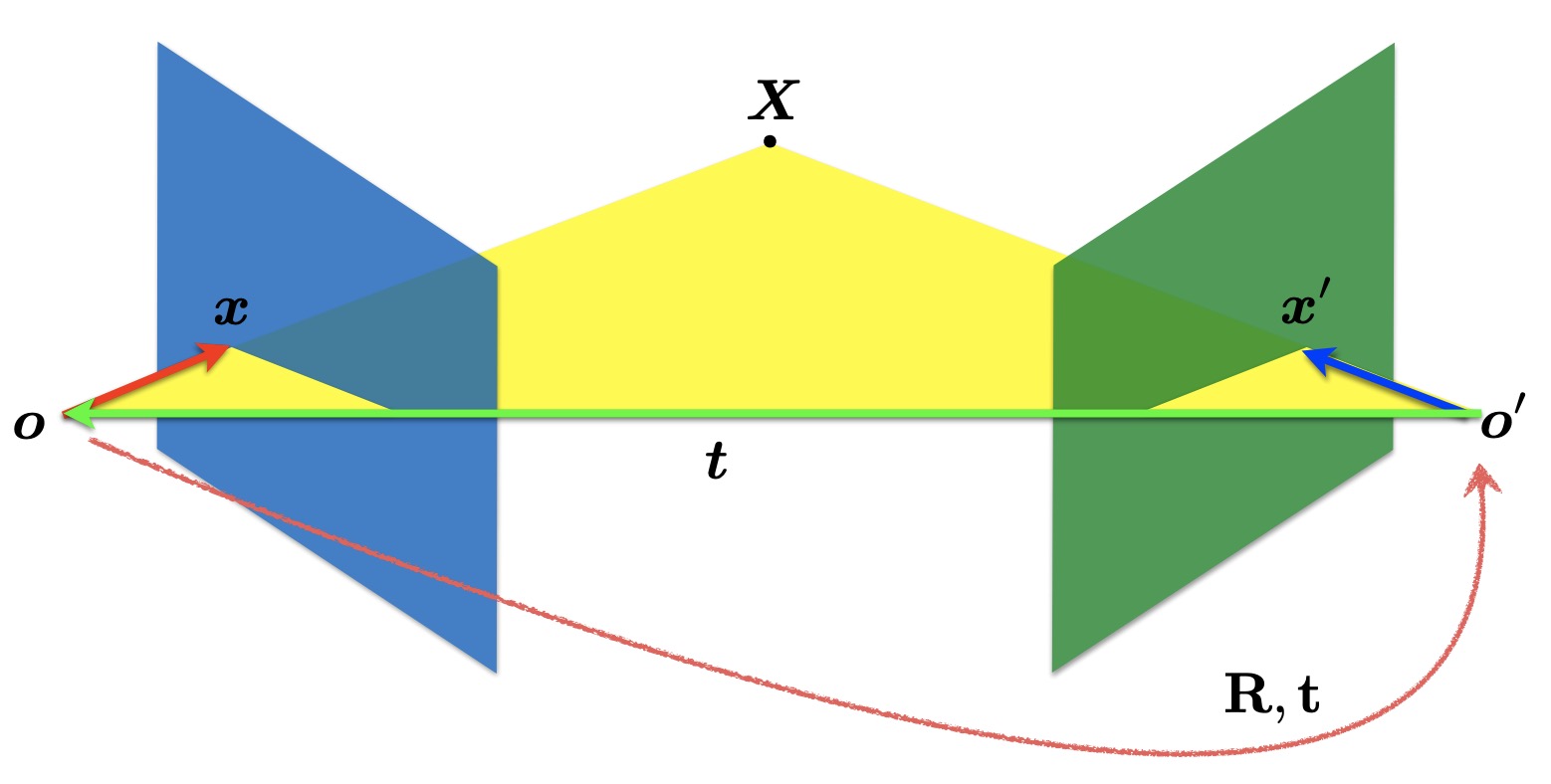
$$x^{\prime}= R(x - t)$$ $$\Rightarrow x^{\prime} R^{-1}= x - t $$

Camera-camera transformation is just world-camera transformation. Since three vectors $x$, $t$, $x^{\prime}$ are co-planar, then

$$x^{\top}(t \times x)=0 $$

$$\Rightarrow (x-t)^{\top}(t \times x)=0 $$

, where $\times$ is cross product. The cross product gives a normal to the plane, and taking the dot product of the normal with any vector in the plane gives $0$.

$$ (x-t)^{\top}(t \times x)=0 $$ $$\Rightarrow (x^{\prime} R^{-1})^{\top}(t \times x)=0 $$ $$\Rightarrow ({x^{\prime}}^{\top} {R^{-1}}^{\top})(t \times x)=0 $$ $$\Rightarrow ({x^{\prime}}^{\top} R)(t \times x)=0 $$

, where $R$ is orthogonal, so $R^{-1} = R^{\top}$. Also, given the cross product, we have

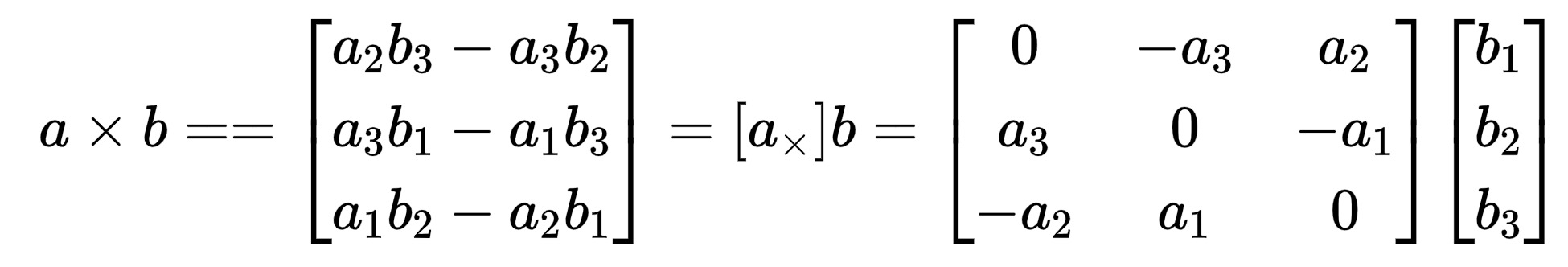
$$({x^{\prime}}^{\top} R)(t \times x)=0 $$ $$\Rightarrow ({x^{\prime}}^{\top} R)([t \times] x)=0 $$ $$\Rightarrow {x^{\prime}}^{\top} R [t \times] x=0 $$ $$\Rightarrow {x^{\prime}}^{\top} E x=0 $$

Properties of Essential Matrix

Longuet-Higgins equation ${x^{\prime}}^{\top} E x=0$
Epipolar lines
- $x^{\prime}$ belongs to epipolar line in the right image defined by $l_r = E x$
- $x$ belongs to epipolar line in the left image defined by $l_l = E^{\top} x^{\prime}$
Epipoles
- ${e^{\prime}}^{\top} E=0$
- $E e=0$

Fundamental Matrix

The Essential matrix operates on image points expressed in normalized camera coordinates. How do we generalize to uncalibrated cameras (i.e. with unknown intrinsic calibrations)?

We need to convert the relationship from physical unit level mapping to pixel-level mapping.

$$ x_c = K^{-1} x_p $$

, where $x$ is camera point and $\hat{x}$ is image point.

$${{x_c}^{\prime}}^{\top} E x_c=0$$ $$\Rightarrow ({{{K^{\prime}}^{-1} {x_p}^{\prime}}})^{\top} E (K^{-1} x_p)=0$$ $$\Rightarrow ({{x_p}^{\prime}}^{\top} {({K^{\prime}}^{-1}})^{\top}) E (K^{-1} x_p)=0$$

$$\Rightarrow ({{x_p}^{\prime}}^{\top}) (({{K^{\prime}}^{-1}})^{\top} E K^{-1}) x_p=0$$ $$\Rightarrow ({{x_p}^{\prime}}^{\top}) F x_p=0$$

Properties of Essential Matrix

Longuet-Higgins equation ${x^{\prime}}^{\top} F x=0$
Epipolar lines
- $x^{\prime}$ belongs to epipolar line in the right image defined by $l_r = F x$
- $x$ belongs to epipolar line in the left image defined by $l_l = F^{\top} x^{\prime}$
Epipoles
- ${e^{\prime}}^{\top} F=0$
- $F e=0$
$F$ has 7 DoF
- $3 * 3$
- Homogenous
- Rank = $2$, $\text{det}(F) = 0$
$F$ contains both intrinsic and extrinsic parameters.

8-point Algorithm

Given a set of matched pairs $\{ x_m, {x_m}^{\prime}\}$, how to estimate $F$?

$${{x_m}^{\prime}}^{\top} F {x_m}=0$$

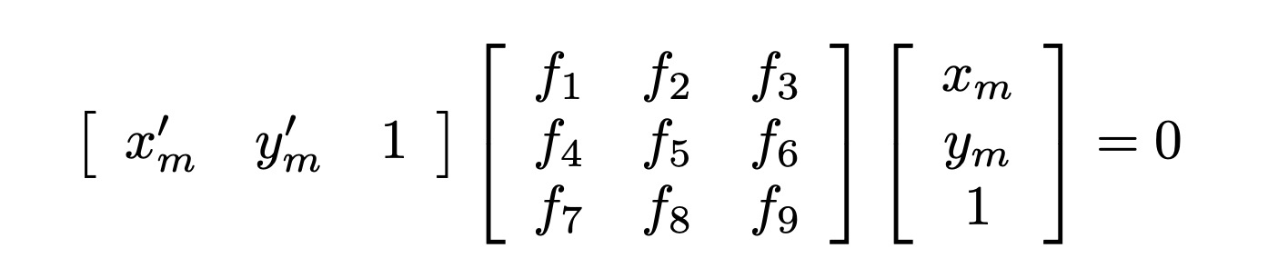
$F$ has $9$ elements, but we don’t care about scaling, so $8$ elements. It turns out it really only has $7$. It uses the fact that the matrix $F$ must be of rank $2$ to fully constrain the matrix. The constraint is not absolutely unique and so three different matrices might be returned (See Zisserman & Hartley’s book for details). Therefore, we need at least $8$ pairs.

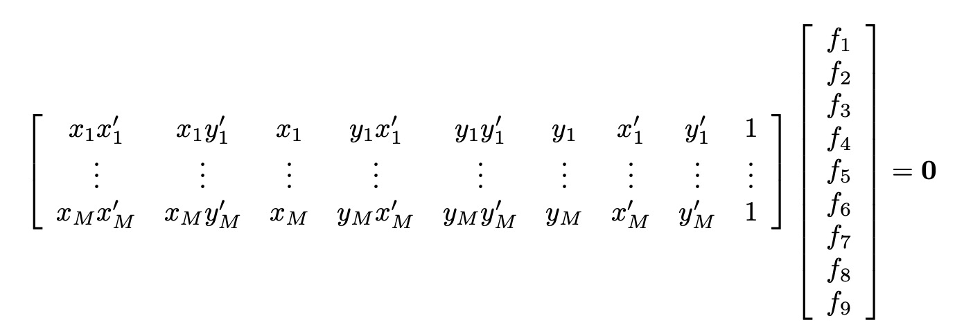
How can we solve the equation $Af=0$? $A$ is constraint matrix. To find $f$, we perform SVD.

Normalize points
Construct the $M * 9$ matrix $A$
Find the SVD of $A^{\top}A$
Entries of $F$ are the elements of column of $V$ corresponding to the least singular value
Enforce rank 2 constraint on $F$
Un-normalize $F$

Pros & Cons

Linear
Easy to implement
Fast
Susceptible to noise

RANSAC

If we use these outlying matches, our estimate $F$ will be wildly inaccurate.

RANdom SAmple Consensus

Sample (randomly) the number of points $s$ required to fit the model
Solve for model parameters using samples
Score by the fraction of inliers within a preset threshold of the model
Repeat 1-3 until the best model is found with high confidence

Note: We call points that are within a certain threshold of the predicted line “inliers”. Everything else is an outlier. Ideally, we want an estimated line/model that maximizes the number of inliers.